Several chart types can represent hierarchical data.
Most common are sunburst, tree and treemap, but sometimes sankey, graph,
even stacked bars can also do the job.
Simple bar charts allow to explore hierarchy levels interactively with
📊 multi-level
drill-down.
An interesting 📊 morphing
demo shows a smooth transition between tree and sunburst charts.
Hierarchical data in R can be represented with different data structures:
- list of lists (or data.frame of data.frames)
- data.frame with parent and child columns
- data.frame with a column for each level (like ‘Titanic’ data)
- data.frame with a record for each leaf (like ‘penguins’ data)
Below are examples for those four data types. Click Show
buttons to see code.
Many users find the second representation most
intuitive and straightforward.
1. List of lists
A simple data structure, but could become difficult to follow with larger trees. echarty can read it as-is, no need for data transformation.
data <- list(
    list(name='Grandpa',
        children= list(
            list(name='Uncle Leo', value=15,
                children= list(list(name='Cousin Jack',value=2),
                    list(name='Cousin Mary',value=5,
                        children=list(list(name='Jackson',value=2))),
                            list(name='Cousin Ben',value=4))),
            list(name='Father', value=10,
               children= list(list(name='Me',value=5),
                    list(name='Brother Peter',value=1))))),
    list(name='Granma Nancy',
        children= list(
            list(name='Uncle Nike',
               children=list(list(name='Cousin Betty',value=1),
                    list(name='Cousin Jenny',value=2)))))
)# -------------------------------------------------

library(echarty)
ec.init(
    series= list(list(
        type= 'sunburst',
        data= data,
        radius= list(0, '90%'),
        labelLayout= list(hideOverlap= TRUE) ))
)
Data frame with nested data.frame children. Similar to
list-of-lists, but with data.frame items, rarely used.
Data transformation is carried out with jsonlite::toJSON
animl <- data.frame(name= "Animals", value= 255)  # top level
animl$children <-
    list(data.frame(name= c("Mammals", "Reptiles","Fish"), value= c(100,90,60)))
animl$children[[1]]$children <- c(
    list(data.frame(name= c("Dogs", "Humans"), value= c( 15, 35))),
    list(data.frame(name= c("Snakes", "Lizards"), value= c(30, 40))),
    list(data.frame(name= c("Sharks"), value = 30)) )
animl$children[[1]]$children[[3]]$children <-
    list(data.frame(name= c("hammerhead", "thresher"), value= c(10,20)))

data <- jsonlite::toJSON(animl)

p <- ec.init(series.param= list(type= 'tree',
        data= data, label= list(offset=c(0, -12)), symbolSize= ec.clmn()  # size by value
))
#p

p <- ec.init(series.param= list(type= 'treemap', data= data, leafDepth= 2))
#p

p <- ec.init(series.param= list(type= 'sunburst',
        # use children instead of root(data) to auto-color descendants
        data= jsonlite::toJSON(animl$children[[1]]),
        radius= c(0, '90%'), label= list(rotate= 'tangential') )
)
#p
2. Data frame with parent-child columns
Data needs to be transformed from data.frame to lists with utility ec.data(format=‘treePC’).
df <- data.frame(
    parents = c("","Reptiles", "Reptiles", "Mammals", "Mammals", "Fish", "Sharks", "Sharks", "Animals", "Animals", "Animals"),
    children = c("Animals", "Snakes", "Lizards", "Dogs", "Humans", "Sharks", "hammerhead", "thresher", "Reptiles", "Mammals", "Fish"),
    value = c(100, 15, 20, 10, 25, 20, 8, 12, 40, 35, 25))
dpc <- ec.data(df, format='treePC')

p <- ec.init(
    series= list(list(type= 'sunburst',
        data= dpc, # =[[1]]$children,
        radius= c(0, '90%'),
        label= list(rotate='tangential'),
        emphasis=list(focus='ancestor') ))
)

p <- ec.init(
    series= list(list(type= 'treemap',
        data=dpc, leafDepth=2,
        label= list(offset = c(0, -12)),
        symbolSize= ec.clmn() )),
    tooltip= list(show= TRUE)
)

#Hierarchy with sankey
edges <- df[-1,] |> rename(source= parents, target= children)
nodes <- list();
for(n in unique(c(edges$source, edges$target)))
    nodes <- append(nodes, list(list(name=n)))
ec.init(
    tooltip= list(show=T),
    series= list(list(type= 'sankey',
        data= nodes,
        edges= ec.data(edges, 'names') ))
) 3. Data frame with a column for each level
A familiar example is the Titanic dataset.
Data is transformed from data.frame to lists with utility
ec.data(format=‘treeTK’)
# build required pathString,value and optional itemStyle columns
df <- as.data.frame(Titanic) |> rename(value= Freq) |> mutate(
    pathString= paste('Titanic\nSurvival', Survived, Age, Sex, Class, sep='/'),
    itemStyle= case_when(Survived=='Yes' ~"color='green'", TRUE ~"color='LightSalmon'")) |>
    select(pathString, value, itemStyle)

dat <- ec.data(df, format='treeTK')
dat[[1]] <- within(dat[[1]], {
    itemStyle <- list(color= 'white'); pct <- 100 })  # customize top

ec.init(
    tooltip= list(formatter= ec.clmn('%@<br>%@%','value','pct')),
    series= list(list(
        type= 'sunburst', radius= c(0, '90%'), label= list(rotate=0),
        # type= 'tree', symbolSize= htmlwidgets::JS("x => {return Math.log(x)*10}",
        # type= 'treemap', upperLabel= list(show=TRUE, height=30), itemStyle= list(borderColor= '#999'), #leafDepth=4,
        data= dat,
        labelLayout= list(hideOverlap= TRUE),
        emphasis= list(focus='none')
    ))
)
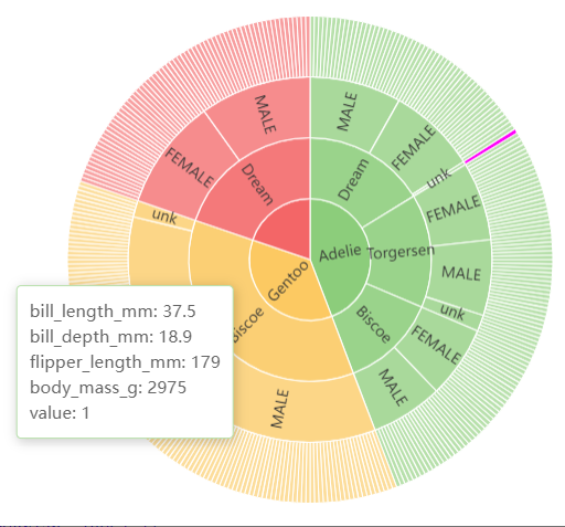
4. Data frame with a record for each leaf
Most popular representation is the penguins multivariate
dataset.
Data transformation is provided by an Extras utility.
See a live demo
of a similar Krane chart with 7K leaves.
Note= " The famous 'penguins' dataset has 344 records in the following format:
species,island,bill_length_mm,bill_depth_mm,flipper_length_mm,body_mass_g,sex
Adelie,Torgersen,39.1,18.7,181,3750,MALE
Adelie,Torgersen,39.5,17.4,186,3800,FEMALE
Adelie,Torgersen,40.3,18,195,3250,FEMALE
Adelie,Biscoe,37.8,18.3,174,3400,FEMALE
Adelie,Dream,37.2,18.1,178,3900,MALE
Adelie,Dream,39.5,17.8,188,3300,FEMALE
Chinstrap,Dream,50.5,18.4,200,3400,FEMALE
Gentoo,Biscoe,46.1,13.2,211,4500,FEMALE
Gentoo,Biscoe,50,16.3,230,5700,MALE"

tmp <- read.csv('https://cdn.jsdelivr.net/gh/mwaskom/seaborn-data@refs/heads/master/penguins.csv')
#data <- getListHierarchy(tmp)   # transform utility is part of Extras
p <- ec.init( tooltip= list(position= c('5%','55%')),
  series.param= list(type= 'sunburst', radius= list(0, 200),
    emphasis= list(focus= 'none', itemStyle= list(color= 'magenta')),
    data= data, labelLayout= list(hideOverlap= TRUE) )
)
#p
